
Yours Ever, Data Chronicles
[kaggle] Bike Sharing Demand: ML 성능 개선 1편 (Ridge, Random Forest, LGBM) 본문
[kaggle] Bike Sharing Demand: ML 성능 개선 1편 (Ridge, Random Forest, LGBM)
Everly. 2022. 7. 1. 07:08직전 포스팅에서는 베이스라인 모델로 선형 회귀(Linear Regression)를 사용해 k-fold를 진행하였고, 검증셋에 대한 RMSLE는 0.9~1 정도로 그렇게 좋은 성능은 얻어내지 못했다.
하지만! 베이스라인 모델이니까 어쩌면 당연하다. 이번에는 다양한 모델들(릿지 회귀, Random Forest, LGBM)을 사용해서 성능이 이전과 얼마나 달라졌는지를 확인하고, 최종 제출까지 해보았다.
참고로 전체 코드는 이 깃허브에서 확인하실 수 있습니다. (ML v.1 파일입니다!)
✔Table of Contents
3. Modeling (성능 개선 편)
캐글에서는 지표로 RMSLE 값을 사용한다고 하였으나, 사이킷런의 metric을 사용하는 관계로 편의를 위해 포스팅에선 MSLE값을 구하는 것으로 하였다. (어차피 MSLE 값에 루트를 씌운 것이 RMSLE 값이므로, MSLE 값을 최소화하도록 구해도 되기 때문에!)
3-1. casual 예측 모델
# X, y 나누기
X_c = train_c.drop(['casual'], axis = 1)
y_c = train_c['casual']
직전 포스팅에서는 선형회귀 모델을 사용했다. 모델을 하나씩 바꿔나가며 MSLE 값이 어떻게 변화하는지를 살펴보자.
1) Ridge
from sklearn.preprocessing import RobustScaler

#릿지
ridge_reg = Ridge()
pipe = make_pipeline(RobustScaler(), ridge_reg)
scores = cross_validate(ridge_reg, X_c, y_c, cv = 5, scoring='neg_mean_squared_error',return_train_score=True)
print("MSLE: {0:.3f}".format(np.mean(-scores['test_score'])))
저번 편에선 StandardScaler, MinMaxScaler만 사용했는데 이번엔 RobustScaler를 사용하였다.
기존에 구한 MSLE 값과 차이가 없어서, 그리드서치를 활용해 하이퍼 파라미터 튜닝을 해보았다.
릿지의 파라미터는 alpha이다.
#릿지 하이퍼 파라미터 튜닝
pipeline = Pipeline([('scaler', RobustScaler()), ('ridge',Ridge())])
params={'ridge__alpha':[5, 10, 15, 20]}
grid_model = GridSearchCV(pipeline, param_grid=params, scoring='neg_mean_squared_error', cv=5)
grid_model.fit(X_c, y_c)
print("MSLE: {0:.3f}".format( -1*grid_model.best_score_))
print('optimal hyperparameter: ', grid_model.best_params_)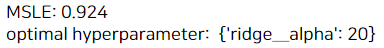
MSLE가 0.924로 조금 향상되었으나, 성능이 크게 좋아지진 않았다.
이번에는 MinMaxScaler로 스케일러를 바꿔보았다.
#릿지에 대해 하이퍼 파라미터 튜닝
pipeline = Pipeline([('scaler', MinMaxScaler()), ('ridge',Ridge())])
params={'ridge__alpha':[5, 10, 15, 20]}
grid_model = GridSearchCV(pipeline, param_grid=params, scoring='neg_mean_squared_error', cv=5)
grid_model.fit(X_c, y_c)
print("MSLE: {0:.3f}".format( -1*grid_model.best_score_))
print('optimal hyperparameter: ', grid_model.best_params_)
MSLE가 0.92로 조금 더 향상되었다. 앞으로는 스케일러를 MinMax로 고정하고 모델을 바꿔보자.
2) Random Forest(랜덤 포레스트)
#rf
np.random.seed(0)
rf =  RandomForestRegressor(n_estimators=500)
#피처에 대해 표준화 진행과 k-fold를 함께 함
pipe = make_pipeline(MinMaxScaler(), rf)
scores = cross_validate(pipe, X_c, y_c, cv=5, scoring='neg_mean_squared_error', return_train_score=True)
print("MSLE: {0:.3f}".format(np.mean(-scores['test_score'])))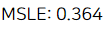
앞서 사용한 선형회귀나 릿지는 그렇게 성능이 뛰어난 모델이 아니다.
랜덤 포레스트를 사용하였더니, 디폴트 모델인데도 MSLE가 0.364로 뛰어나게 향상되었다.
더 좋은 모델을 위해 그리드서치로 하이퍼 파라미터 튜닝을 해보았다.
랜덤 포레스트부터는 하이퍼파라미터가 아주 다양하기에 어떤 파라미터를 선택할지도 주의해야 한다. (게다가 시간도 오래 걸리니 주의!)
파라미터에 대한 자세한 정보는 밑의 사이킷런 페이지에서 확인할 수 있다. 나는 임의로 몇 가지 선택해서 튜닝해보았다.
sklearn.ensemble.RandomForestRegressor
Examples using sklearn.ensemble.RandomForestRegressor: Release Highlights for scikit-learn 0.24 Release Highlights for scikit-learn 0.24, Combine predictors using stacking Combine predictors using ...
scikit-learn.org
#rf 하이퍼 파라미터 튜닝
pipeline = Pipeline([('scaler', MinMaxScaler()), ('rf',RandomForestRegressor())])
params={'rf__max_depth': [5,10,None],
       'rf__min_samples_leaf': [1,3],
       'rf__min_samples_split': [2, 3],
        'rf__n_estimators': [500, 1000]}
grid_model = GridSearchCV(pipeline, param_grid=params, scoring='neg_mean_squared_error', cv=5, n_jobs = 5, verbose=True)
grid_model.fit(X_c, y_c)
print("MSLE: {0:.3f}".format( -1*grid_model.best_score_))
print('optimal hyperparameter: ', grid_model.best_params_)
위의 코드 실행 시 시간이 꽤 오래 걸린다. (위의 에러 메세지를 보면 약 18분 걸렸다,,)
성능은 0.364에서 0.358로 소폭 향상되었다.
3) LGBM
#LGBM
lgbm = LGBMRegressor(n_estimators = 500, objective = 'regression')

#피처에 대해 표준화 진행과 k-fold를 함께 함
pipe = make_pipeline(MinMaxScaler(), lgbm)
scores = cross_validate(pipe, X_c, y_c, cv=5, scoring='neg_mean_squared_error', return_train_score=True)
print("MSLE: {0:.3f}".format(np.mean(-scores['test_score'])))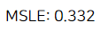
마지막으로는 모델링에서 내가 애용하는 LGBM(Lightgbm)을 사용해보았다.
앞의 랜덤 포레스트에서 그리드서치로 18분이나 걸려서 0.358을 얻기가 무색하게, 디폴트로만 0.332라는 좋은 성능이 나왔다. ㅎㅎ..
하지만 LGBM이 언제나 가장 좋은 성능을 내는 것은 아니라서 주의가 필요하다.
LGBM도 좀 더 성능향상을 위해 하이퍼 파라미터 튜닝을 했다. 이 모델도 파라미터가 아주 많기 때문에 어떤 것을 선택할지 주의가 필요하다. 파라미터는 여기서 확인할 수 있다.
lightgbm.LGBMRegressor — LightGBM 3.3.2.99 documentation
Build a gradient boosting model from the training set (X, y). Note Custom eval function expects a callable with following signatures: func(y_true, y_pred), func(y_true, y_pred, weight) or func(y_true, y_pred, weight, group) and returns (eval_name, eval_res
lightgbm.readthedocs.io
#하이퍼 파라미터 튜닝
pipeline = Pipeline([('scaler', MinMaxScaler()), ('lgbm',LGBMRegressor(objective='regression'))])
params={'lgbm__learning_rate': [0.001, 0.01, 0.1],
       'lgbm__max_depth': [5, 10],
       'lgbm__reg_lambda':[0.1, 1],
       'lgbm__subsample': [0.5, 1],
       'lgbm__n_estimators': [500, 1000]}
grid_model = GridSearchCV(pipeline, param_grid=params, scoring='neg_mean_squared_error', cv=5, n_jobs = 5, verbose=True)
grid_model.fit(X_c, y_c)
print("MSLE: {0:.3f}".format( -1*grid_model.best_score_))
print('optimal hyperparameter: ', grid_model.best_params_)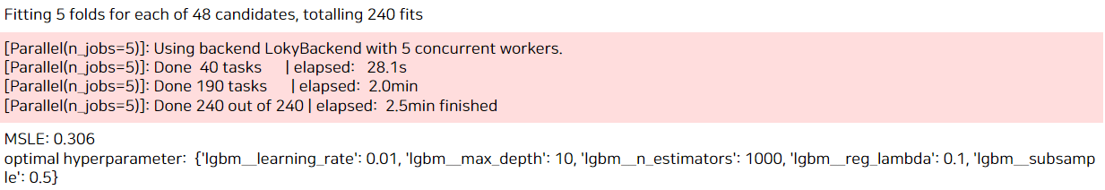
결과는 0.306으로 가장 좋은 성능이었다. LGBM은 가볍기 때문에 약 3분 정도 걸려 그리드서치가 완료되었다.
여기서 max_depth 값이 가장 큰 10이 가장 최적이라고 나와서, 범위를 10과 15로 크게 하여 다시 실행하였다.
#하이퍼 파라미터 튜닝
pipeline = Pipeline([('scaler', MinMaxScaler()), ('lgbm',LGBMRegressor(objective='regression', learning_rate = 0.01, subsample = 0.5))])
params={'lgbm__max_depth': [10, 15],
       'lgbm__reg_lambda':[0.1, 1],
       'lgbm__n_estimators': [500, 1000]}
grid_model = GridSearchCV(pipeline, param_grid=params, scoring='neg_mean_squared_error', cv=5, n_jobs = 5, verbose=True)
grid_model.fit(X_c, y_c)
print("MSLE: {0:.3f}".format( -1*grid_model.best_score_))
print('optimal hyperparameter: ', grid_model.best_params_)
max_depth는 15가 최적으로 나왔고, n_estimators도 500으로 줄어들었다. 성능은 0.306으로 동일!
그래서 최종적으로는 다음의 파라미터를 사용해 최종 모델링에 사용하기로 결정했다.
lgbm = LGBMRegressor(n_estimators = 500, objective = 'regression', learning_rate = 0.01, subsample = 0.5, max_depth = 15, reg_lambda = 0.1)
3-2. registered 예측 모델
# X, y 나누기
X_r = train_re.drop(['registered'], axis = 1)
y_r = train_re['registered']
이번에는 registered 모델을 만들어보았다. 앞에서 여러 모델을 써봤지만 LGBM이 가장 좋았기에 곧바로 LGBM 모델을 적합해보았다.
#LGBM
lgbm = LGBMRegressor(n_estimators = 500, objective = 'regression')

#피처에 대해 표준화 진행과 k-fold를 함께 함
pipe = make_pipeline(MinMaxScaler(), lgbm)
scores = cross_validate(pipe, X_r, y_r, cv=5, scoring='neg_mean_squared_error', return_train_score=True)
print("MSLE: {0:.3f}".format(np.mean(-scores['test_score'])))
역대급으로 좋은 성능이 나왔다. 파라미터 튜닝도 안 했는데 0.182가 나왔다.
하지만 과적합된 것일 수도 있다. test set에 대해 예측했을 때도 이렇게 좋은 결과가 나오리란 법은 없으니까 말이다.
아무튼 조금 더 튜닝을 해보았다.
#하이퍼 파라미터 튜닝
pipeline = Pipeline([('scaler', MinMaxScaler()), ('lgbm',LGBMRegressor(objective='regression', learning_rate = 0.1, subsample = 0.5))])
params={'lgbm__max_depth': [3, 5, 7],
       'lgbm__reg_lambda':[0.1, 1],
       'lgbm__n_estimators': [300, 500]}
grid_model = GridSearchCV(pipeline, param_grid=params, scoring='neg_mean_squared_error', cv=5, n_jobs = 5, verbose=True)
grid_model.fit(X_r, y_r)
print("MSLE: {0:.3f}".format( -1*grid_model.best_score_))
print('optimal hyperparameter: ', grid_model.best_params_)
결과는 0.168로 좀 더 향상되었다.
그래서 최종 파라미터는 다음의 것들을 사용하기로 결정!
LGBMRegressor(n_estimators = 500, objective = 'regression', learning_rate = 0.1, max_depth = 3, reg_lambda = 0.1, subsample = 0.5)
4. Predict Test data
이제 본격적으로 만들어진 모델을 활용해 test data에 대해 예측하고, 최종 제출해보자!
먼저, test data를 앞의 train data처럼 가공하였다.
test['year'] = test['datetime'].dt.year
test['month'] = test['datetime'].dt.month
test['hour'] = test['datetime'].dt.hour
test['dayofweek'] = test['datetime'].dt.dayofweek

#datetime 삭제
del test['datetime']

test.head()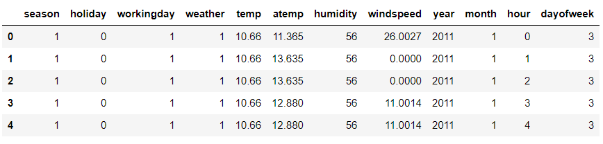
#카테고리 변수 생성
cate_name = ['weather', 'season', 'year', 'month', 'hour', 'dayofweek']

for c in cate_name:
    test[c] = test[c].astype('category')
test.dtypes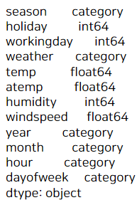
이제는 test data에 casual 예측모델을 사용해 casual을 예측하고,
registered 예측모델을 사용해 registered를 예측해보자.
최종 결과는 예측 casual + 예측 registered를 더한 값이다!
4-1. casual 예측하기
# 피처 표준화
minmax = MinMaxScaler()
minmax.fit(X_c) #훈련셋 모수 분포 저장
X_c_scaled = minmax.transform(X_c)
X_test_scaled = minmax.transform(test)
먼저 앞서 사용했던 것처럼 스케일링을 test data에도 시켜줘야 한다.
MinMax Scaler를 사용하였으며, 먼저 fit 메서드로 train data의 분포를 저장한다.
그 후, transform 메서드로 train data, test data 각각에 대해 스케일링해준다.
Q. 근데 앞에서 train data는 스케일링 해준거 아니에요? 왜 또 해줘요?
→ train data 전체에 대해 스케일링 해준 게 아니기 때문에 해줘야 한다. 앞에서는 train data를 k-fold하여 훈련셋/검증셋으로 나누었고 이에 대해 스케일링을 해준 것!
그리고 여기서 하는 것은 train data 전체 모수를 바탕으로 train data/test data 각각에 스케일링을 해준 것이다.
# 최종 파라미터 튜닝된 모델로 학습
lgbm1 = LGBMRegressor(n_estimators = 500, objective = 'regression',
                    learning_rate = 0.01, subsample = 0.5, max_depth = 15, reg_lambda = 0.1, ranodm_state = 99)

# 학습
lgbm1.fit(X_c_scaled, y_c)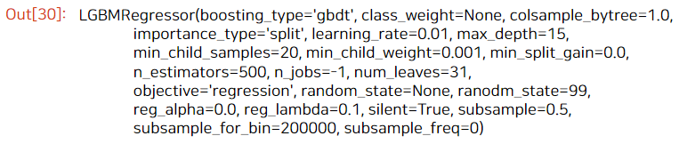
# test에 대해 예측
pred_c = lgbm1.predict(X_test_scaled)
fpred_c = np.expm1(pred_c) #로그변환 값을 풀어줌
앞에서 만든 casual 예측모델을 활용해 test data에 대해 예측해주었다.
그리고 만들어진 결과는 pred_c이며, 이 값은 로그값으로 되어 있기 때문에 최종 결과로는 np.expm1 을 활용해 로그값을 풀어줘야 한다.
여기서 우리가 사용한 변수들 중에 어떤 게 가장 중요한 변수였는지를 확인해보자!
#lgbm1 모델의 feature importance
imp_casual = pd.DataFrame({'feature': test.columns,
                                    'coefficient': lgbm1.feature_importances_})
imp_casual = imp_casual.sort_values(by = 'coefficient', ascending = False)

plt.barh(imp_casual['feature'], imp_casual['coefficient'])
plt.show()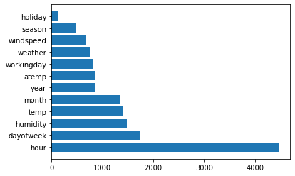
EDA 결과를 통해 hour가 가장 중요한 변수라고 했는데, LGBM 모델도 정말 엄청 중요도가 높게 설정하였다.
그 다음으로는 요일 > 습도 > 온도 > month > year 등이 중요도가 높았다.
4-2. registered 예측하기
# 피처 표준화
minmax = MinMaxScaler()
minmax.fit(X_r) #훈련셋 모수 분포 저장
X_r_scaled = minmax.transform(X_r)
X_test_scaled = minmax.transform(test)
마찬가지로 스케일링을 해준다. 앞에서 설명했으므로 넘어간다.
# 최종 파라미터 튜닝된 모델로 학습
lgbm2 = LGBMRegressor(n_estimators = 500, objective = 'regression',learning_rate = 0.1, max_depth = 3, reg_lambda = 0.1, subsample = 0.5, random_state = 99)
# 학습
lgbm2.fit(X_r_scaled, y_r)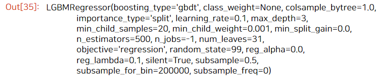
# test에 대해 예측
pred_re = lgbm2.predict(X_test_scaled)
fpred_re = np.expm1(pred_re) #로그변환 값을 풀어줌

#lgbm2 모델의 feature importance
imp_re = pd.DataFrame({'feature': test.columns,
                                    'coefficient': lgbm2.feature_importances_})
imp_re = imp_re.sort_values(by = 'coefficient', ascending = False)

plt.barh(imp_re['feature'], imp_re['coefficient'])
plt.show()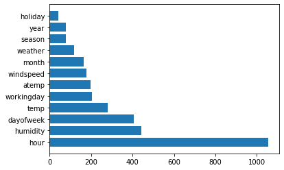
만들어진 모델로 test data에 대해 예측을 해주었고, 피처별 중요도를 뽑아보았다.
registered 모델도 역시 hour의 기여도가 높았으며, 그 다음이 습도 > 요일 > 온도 > workingday 등이었다.
4-3. 최종 결과
이제 만들어진 예측치들을 합치면 끝!
test['casual_pred'] = fpred_c
test['re_pred'] = fpred_re
test['count'] = test['casual_pred'] + test['re_pred']
test.head()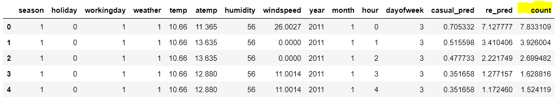
이렇게 하여 test 데이터의 count 값이 예측되었다.
이제 submission 데이터를 가져와서 count 값을 넣고 제출을 완료해보자.
# submission 가져오기
sub = pd.read_csv('data/sampleSubmission.csv')
del sub['count']
sub['count'] = test['count']
sub.head()
sub.to_csv('Submission_sy_0.csv', index=False)
캐글 제출결과는..
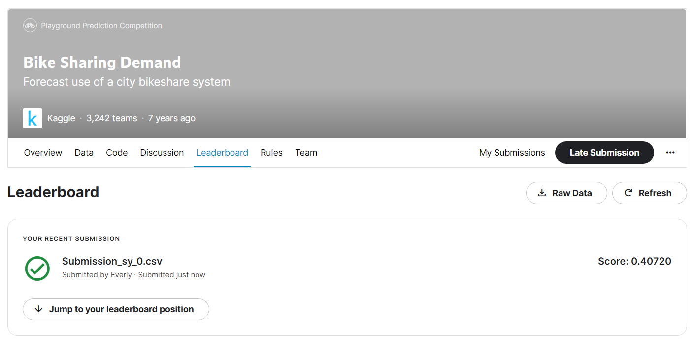
이렇게 0.40720 이라는 점수가 나왔다.
1등의 점수가 약 0.33이었고, 이미 지난 대회라 나의 순위를 확인할 수는 없지만, 이정도면 나쁘지 않은 성적을 받았다고 볼 수 있다.
여기서 끝이 아니라, 조금 더 방법을 바꿔가며 성능을 또 한번 개선해보았다.
casual/registered 나눠서 예측하는 게 아니라 count를 예측해보거나, season과 month 변수가 겹치므로 둘 중 하나만 사용해서 성능을 측정해보거나 하는 식이다.
각각 깃허브에 v.2~v.5 버전으로 올려두었으며, 다음 포스팅에서는 이렇게 방법을 바꿔본 이유와 개선된 성능에 대해 알아보자 :)
'Data Science > Kaggle' 카테고리의 다른 글
| [kaggle] Bike Sharing Demand: ML 성능 개선 3편 (머신러닝 결측치 처리) (2) | 2022.07.03 |
|---|---|
| [kaggle] Bike Sharing Demand: ML 성능 개선 2편 (변수 선택) (0) | 2022.07.02 |
| [kaggle] Bike Sharing Demand: Baseline Model 2편 (pipeline, k-fold, scaling) (0) | 2022.06.30 |
| [kaggle] Bike Sharing Demand: Baseline Model 1편 (데이터 전처리) (2) | 2022.06.30 |
| [kaggle] Bike Sharing Demand: EDA 2편 (0) | 2022.06.25 |


